A Python Demo for MD simulation of Lennard-Jones Fluid in NVT Ensemble

一个简单的demo,用Python实现在NVT系综中Lennard-Jones流体的分子动力学模拟。原理见Molecular Dynamics in NVT ensemble一文。

Code: 参数设置和变量初始化

1
2
3
4
5
6
7
8
9
10
11
12
13
14
15
16
17
18
19
20
21
22
23
24
25
26
27
28
29
30
31
32
33
34
35
36
37
38
39
40
41
42
43
44
45
46
47
48
49
50
51
52
53
54
55
56
57
58
59
60
61
62
63
64
65
66
67
68
69
70
71
72
73
74
75
76
77
78
79
80
81
82
83
84
85
86
87
88
89
90
91
92
93
94
95
96
97
98
99
100
101
102
103
104
105
106
107
108
109
110
111
112
113
114
115
116
117
118
119
120
121
122
123
124
125
126
127
128
129
130
131
132
133
134
import numpy as np
import matplotlib.pyplot as plt
from math import sinh, exp, sqrt, pi
from numpy import log, sin, cos

def setParm(dti,nthermoi,nstepi,Ni,T0i,Mi,taoi):
'''
:: setParm(dti,nthermoi,nstepi,T0i,Mi,taoi,x0i,mi,omegai)
set up the simulation parameters directly

dti: the time step (ps)
nthermoi: the proportion that dt/dt(NHC)
nstepi: the number of the simulation steps
Ni: the number of particles
T0i: the target temperature (K)
Mi: the number of thermostats
taoi: the character time scale 'tao'(ps)
'''
global k
k=0.0083144621 # MD单位下的玻尔兹曼常数
#注意:函数内可以使用全局变量但不能修改,除非函数开头加global关键字声明
global dt
global nthermo
global dtmo
global nstep
global T0
global M
global Q
global N

print("Set up the simulation paramaters")
dt=dti
nthermo=nthermoi
dtmo=np.zeros(7)
for ntt in np.arange(7):
dtmo[0]= 0.784513610477560*dt/nthermo
dtmo[6]= dtmo[0]
dtmo[1]= 0.235573213359357*dt/nthermo
dtmo[5]= dtmo[1]
dtmo[2]= -1.17767998417887*dt/nthermo
dtmo[4]= dtmo[2]
dtmo[3]= (1-(0.784513610477560-0.235573213359357+1.17767998417887)*2)*dt/nthermo
nstep=nstepi
N=Ni
T0=T0i
M=Mi
tao=taoi
Q=np.zeros(M)
Q[0]=3*N*k*T0*tao*tao
for m in np.arange(1,M):
Q[m]=k*T0*tao*tao


def setBC():
'''
setting up the boundary condition
'''
global pbc
bcType=input("the type of periodic boundary condition (e.g. 'cubic','rectangle','noPBC'): ")
if bcType!="noPBC":
global lxbox
global lybox
global lzbox
if bcType=="cubic":
lxbox=float(input("the length of the cubic box (nm): "))
lybox=lxbox
lzbox=lxbox
else:
lxbox=float(input("the x length of the box (nm): "))
lybox=float(input("the y length of the box (nm): "))
lzbox=float(input("the z length of the box (nm): "))
pbc=[bcType,lxbox,lybox,lzbox]
else:
pbc=[]
def initial_position():
'''
initialization of the particle positions: a N*3 array
only for monatomic system with single componment, N=a^3
'''
global r
r=np.zeros([N,3])
a=pow(N,1/3)
for i in np.arange(1,N+1):
r[i-1]=np.array([(i%(a*a))%a,(i%(a*a))//a,i//(a*a)])*lxbox/a
r[i-1][0]=r[i-1][0]-lxbox*round(r[i-1][0]/lxbox)
r[i-1][1]=r[i-1][1]-lybox*round(r[i-1][1]/lybox)
r[i-1][2]=r[i-1][2]-lzbox*round(r[i-1][2]/lzbox)

def initial_velocity(Ti):
'''
initialization of the particle velocity according to the MB distribution (it's unnecessary)

'''
global velocity
global KE
global T
velocity = np.zeros([N,3])
T=Ti
sigma=sqrt(k*T/m[0])
np.random.seed(19015601)
ran1 = np.random.rand(N)
ran2 = np.random.rand(N)
ran3 = np.random.rand(N)
velocity[:,0]= sigma*np.sqrt(-2*log(1-ran2))*cos(2*pi*ran1)
velocity[:,1]= velocity[:,0]/cos(2*pi*ran1)*sin(2*pi*ran1)
velocity[:,2]=sigma*np.sqrt(-2*log(1-ran2))*cos(2*pi*ran3)

sumv=sum(sum(velocity))
velocity=velocity-sumv/(N*3)
sumv2=0
for i in np.arange(N):
sumv2=sumv2+sum(velocity[i]*velocity[i])*m[i]
fs=sqrt(3*N*k*T/sumv2)
velocity*=fs

KE=0.5*3*N*k*T


def initial_G():
global G
G=np.zeros(M)
G[0]=3*N*k*(T-T0)
for ng in np.arange(1,M):
G[ng]=(Q[ng-1]*vEta[ng-1]*vEta[ng-1]-k*T0)/Q[ng]
def initial_nhc(label):
global eta
global vEta
if label=="random":
np.random.seed(19588801)
eta = np.random.rand(M)
vEta = np.random.rand(M)
elif label=="zero":
eta=np.zeros(M)
vEta=np.zeros(M)

Code: 单步积分器

1
2
3
4
5
6
7
8
9
10
11
12
13
14
15
16
17
18
19
20
21
22
23
24
25
26
27
28
29
30
31
32
33
34
35
36
37
38
39
40
41
42
43
44
45
46
47
48
49
50
51
52
53
54
55
56
57
58
59
60
61
62
63
64
65
66
67
68
69
70
71
72
73
74
75
76
77
78
def NHCstep():
'''
solve the Nosé-Hoover Chain equations using "explict rversible intergrators in a single step
changed global variable:particle positions N*3 : r; particle velosity N*3: velocity; physical forces N*3: Force;
M* eta; M* vEta; thermostat forces M* G ; potential energy UE.
kinetic energy KE, instantaneous temperature T (but not be calculated in this function)
'''
for nweight in np.arange(7):
for ns in np.arange(nthermo):
Soperator(dtmo[nweight])
vverletStep()
for nweight in np.arange(7):
for ns in np.arange(nthermo):
Soperator(dtmo[nweight])
def Soperator(tm):
'''
tm : the time step of each weight in the exp(iLnhc)
'''
global vEta
global G
global eta
global velocity
global T
global KE

vEta[M-1]+=G[M-1]*tm/4
for jj in np.flipud(np.arange(M-1)): #逆向序列 [M-2,M-3,...,0]
vt_tmp=tm/8*vEta[jj+1]
vEta[jj]*=exp(-vt_tmp)
vEta[jj]+=tm/4*G[jj] #exect: *sinh(vt_tmp)/(vt_tmp)
vEta[jj]*=exp(-vt_tmp)
G[jj+1]=(Q[jj]*vEta[jj]*vEta[jj]-k*T0)/Q[jj+1]
for j in np.arange(M):
eta[j]+=tm/2*vEta[j]
KE=0
for i in np.arange(N):
velocity[i]*=exp(-tm/2*vEta[0])
KE+= m[i]*sum(velocity[i]*velocity[i])
T=KE/(3*N*k)
G[0]=3*N*k*(T-T0)
KE*=0.5
for j in np.arange(M-1):
vt_tmp=tm/8*vEta[j+1]
vEta[j]*=exp(-vt_tmp)
vEta[j]+=tm/4*G[j] #exect: *sinh(vt_tmp)/(vt_tmp)
vEta[j]*=exp(-vt_tmp)
G[j+1]=(Q[j]*vEta[j]*vEta[j]-k*T0)/Q[j+1]
vEta[M-1]+=G[M-1]*tm/4

def vverletStep():
global velocity
global r
global T
global KE
KE=0

if pbc!=[]:
for i in np.arange(N):
velocity[i]+=dt/2*Force[i]/m[i]
r[i]+=dt*velocity[i]
r[i][0]=r[i][0]-lxbox*round(r[i][0]/lxbox)
r[i][1]=r[i][1]-lybox*round(r[i][1]/lybox)
r[i][2]=r[i][2]-lzbox*round(r[i][2]/lzbox)
LJforce()
for i in np.arange(N):
velocity[i]+=dt/2*Force[i]/m[i]
KE+=m[i]*sum(velocity[i]*velocity[i])
else:
for i in np.arange(N):
velocity[i]+=dt/2*Force[i]/m[i]
r[i]+=dt*velocity[i]
LJforce()
for i in np.arange(N):
velocity[i]+=dt/2*Force[i]/m[i]
KE+=m[i]*sum(velocity[i]*velocity[i])
T=KE/(3*N*k)
G[0]=3*N*k*(T-T0)
KE*=0.5

力与势能的计算

  • Lennard-Jones Potential

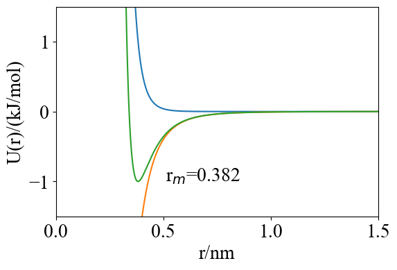
\[ U^{LJ}(r_{ij})=4\epsilon \bigl(\frac{\sigma^{12}}{r_{ij}^{12}}-\frac{\sigma^6}{r_{ij}^6}\bigr)\\ r_{ij}=\sqrt{(x_i-x_j)^2+(y_i-y_j)^2+(z_i-z_j)^2} \]

Force \[ Fx_i=-\frac{\partial U^{LJ}(r_{ij})}{\partial x_i}=4\epsilon \bigl(\frac{12\sigma^{12}}{r_{ij}^{13}}-\frac{6\sigma^6}{r_{ij}^7}\bigr)\cdot\frac{x_i}{r_{ij}} \] Extreme point \[ r_m=\sqrt[6]{2}\,\sigma \]

1
2
3
4
5
6
7
8
9
10
11
12
13
14
15
16
17
import matplotlib.pyplot as plt
import numpy as np
plt.figure(dpi=100)
r=np.linspace(0.3,1.5,1000)
u12=4*(0.3405/r)**12
u6=-4*(0.3405/r)**6
u=u12+u6
plt.xlabel("r/nm")
plt.xlim(0,1.5)
plt.ylabel("U(r)/(kJ/mol)")
plt.ylim([-1.5,1.5])
plt.plot(r,u12,label="r12 repulsive potential")
plt.plot(r,u6,label="r6 attractive potential")
plt.plot(r,u,label="Lennard-Jones potential")
plt.text(0.51,-1,"r$_m$={:.3f}".format(0.3405*pow(2,1/6)))
plt.show()

image-20250207011425727

1
2
3
4
5
6
7
8
9
10
11
12
13
14
15
16
17
18
19
20
21
22
23
24
25
26
27
28
29
30
31
32
33
34
35
36
37
38
39
40
41
42
43
44
45
46
47
48
49
50
51
52
53
def LJtopology(elji,sigmalji,rci):
global sigmalj
global sigmalj6
global elj
global rc2 # cutoff radial
global ecut

elj=elji
sigmalj=sigmalji
rc=rci
rc2=rc*rc
sigmalj6=sigmalj**6
sir=sigmalj6/(rc2**3)
ecut=4*elj*sir*(sir-1)

def LJforce():
global Force
global UE

'''
simple cutoff sheme, rc <= min(lbox)/2, calculate Force and Potential energy with minimum image convention rule.
'''
Force=np.zeros([N,3])
UE=0
if pbc==[]:
for i in np.arange(N-1):
for j in np.arange(i+1,N):
xr=r[i]-r[j]
r2=sum(xr*xr)
if r2 < rc2:
r2i=1/r2
r6i=r2i**3
r8i=r6i*r2i
ff=48*elj*sigmalj6*r8i*(sigmalj6*r6i-0.5)*xr
Force[i]+=ff
Force[j]+=-ff
UE+=4*elj*sigmalj6*r6i*(sigmalj6*r6i-1)-ecut
else:
for i in np.arange(N-1):
for j in np.arange(i+1,N):
xr=r[i]-r[j]
xr[0]=xr[0]-lxbox*round(xr[0]/lxbox)
xr[1]=xr[1]-lybox*round(xr[1]/lybox)
xr[2]=xr[2]-lzbox*round(xr[2]/lzbox)
r2=sum(xr*xr)
if r2 < rc2:
r2i=1/r2
r6i=r2i**3
r8i=r6i*r2i
ff=48*elj*sigmalj6*r8i*(sigmalj6*r6i-0.5)*xr
Force[i]+=ff
Force[j]+=-ff
UE+=4*elj*sigmalj6*r6i*(sigmalj6*r6i-1)-ecut

参数设置

  • Simulation parameters: the time step (ps): 0.01 the proportion that dt/dt(NHC): 20 the number of the simulation steps: 10000 the number of particles: 216 the target temperature (K): 119.8 the number of thermostats: 2 the character time scale \(\tau\) (ps): 0.2

  • Boundary Condition: cubic box lbox= 2.04 nm

  • Topology: 216 Ar atoms, mass 39.94 g/mol LJ_epsilon: 0.99607 kJ/mol LJ_sigma: 0.3405 nm Cutoff radial: 1.0 nm

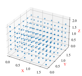
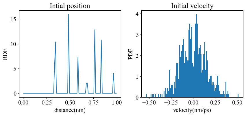
  • Initialization: positions: put the particles on the cubic lattice velocities: use Box-Miller method sampling the MB distribution at Ti=110 K thermostat variables: zeros

  • Dump the T,UE,KE,velocities and positions every step!

Code:模拟与数据存储

1
2
3
4
5
6
7
8
9
10
11
12
13
14
15
16
17
18
19
20
21
22
23
24
25
26
27
28
29
30
31
32
33
34
35
36
37
38
#setParm(dti, nthermoi, nstepi,Ni, T0i, Mi, taoi)
setParm(0.01, 20, 10000, 216, 119.8, 2, 0.2)
setBC()
LJtopology(0.99607, 0.3405, 1.0)
mass=39.94
global m
m=np.ones(N)*mass
#初始化
initial_position()
initial_velocity(110)
LJforce()
initial_nhc("zero")
initial_G()
#模拟
Ts=np.zeros(nstep+1)
KEs=np.zeros(nstep+1)
UEs=np.zeros(nstep+1)
vstore=np.zeros([nstep+1,N,3])
xstore=np.zeros([nstep+1,N,3])
times=np.zeros(nstep+1)
print("Simulation start!")
global time
global ncount
ncount=0
time=0
while ncount <= nstep:
Ts[ncount]=T
KEs[ncount]=KE
UEs[ncount]=UE
xstore[ncount]=r
vstore[ncount]=velocity
times[ncount]=time
if ncount%100==0:
print([ncount,T,KE,UE])
NHCstep()
time=ncount*dt
ncount=ncount+1
print("Simulation finish!")
Set up the simulation paramaters
the type of periodic boundary condition (e.g. 'cubic','rectangle','noPBC'): cubic
the length of the cubic box (nm): 2.04
Simulation start!
[0, 110, 296.327429244, -789.1019846977582]
... ...
Simulation finish!
1
2
3
4
5
6
7
8
9
10
11
12
13
14
15
16
17
18
19
#dump temperature, kinetic, potential and total energy
file=open("./LJsim1_log.txt",mode='w')

for line in np.arange(10001):
file.writelines("{nsteps} {time:.2f} {T:.14f} {KE:.14f} {UE:.14f} {TE:.14f}\n".format(nsteps=line,time=times[line],T=Ts[line],KE=KEs[line],UE=UEs[line],TE=KEs[line]+UEs[line]))
file.close()

vfile=open("./LJsim1_v.txt",mode='w')
for step in np.arange(10001):
vfile.writelines("{nsteps} {time:.2f}\n".format(nsteps=step,time=times[step]))
for i in np.arange(216):
vfile.writelines("{vx} {vy} {vz}\n".format(vx=vstore[step,i,0],vy=vstore[step,i,1],vz=vstore[step,i,2]))
vfile.close()
xfile=open("./LJsim1_x.txt",mode='w')
for step in np.arange(10001):
xfile.writelines("{nsteps} {time:.2f}\n".format(nsteps=step,time=times[step]))
for i in np.arange(216):
xfile.writelines("{xx} {xy} {xz}\n".format(xx=xstore[step,i,0],xy=xstore[step,i,1],xz=xstore[step,i,2]))
xfile.close()
1
2
3
4
5
6
#用pickle方法读写数据
import pickle
with open('LJsim1_vstore.pickle', 'wb') as f:
pickle.dump(vstore, f)
with open('LJsim1_xstore.pickle','wb') as f:
pickle.dump(xstore,f)

数据分析与可视化

径向分布函数 (RDF)

  • 原子b对原子a的径向分布函数定义为:

\[ g_{ab}(r)=\frac{P_b(r)}{4\pi\rho_br^2dr} \]

其中\(P_b(r)\)是原子b出现在离原子a距离为\([r,r+dr)\)的球形壳层中的概率。故径向分布函数就是径向概率密度除以原子b的平均密度,归一化到\(N_b\)。在无限远处 \(g_{ab}(\infty)=\rho_b\)。 实际计算时,首先设定最大距离 \(r_{max} (<\frac{1}{2}L_{box})\) 和区间数 \(N_r\) 。将 \([0,r_{max})\) 分为宽度为\(\Delta r=r_{max}/N_r\)\(N_r\) 个小区间,对轨迹的每一帧、每个a、b原子对,统计距离落在区间 \([r_i,r_i+dr)\) 的频数 \(h_{ab}(i)\)。可用下式获取小区间的index: \[ i=int(\frac{r}{\Delta r}) \] 最终径向分布函数可用下式计算: \[ g_{ab}(r_i)=\frac{h_{ab}(r_i)}{4\pi\rho_br_i^2\Delta rN_{conf}N_a} \]

1
2
3
4
5
6
7
8
9
10
11
12
13
14
15
16
17
18
19
20
21
22
23
24
25
26
27
28
29
30
#计算RDF
def RDF(xtrj,rmax,nr):
'''
xtrj: trjectory
rmax: maximum distance
nr: the number of intervals
'''
Nconf=len(xtrj)
Na=len(xtrj[0])
rho=Na/(lxbox*lybox*lzbox)
dr=rmax/nr
disr=np.zeros(nr)
rdf=np.zeros(nr)
for ncg in np.arange(Nconf):
for i in np.arange(Na-1):
for j in np.arange(i+1,Na):
xr=xtrj[ncg,i]-xtrj[ncg,j]
xr[0]=xr[0]-lxbox*round(xr[0]/lxbox)
xr[1]=xr[1]-lybox*round(xr[1]/lybox)
xr[2]=xr[2]-lzbox*round(xr[2]/lzbox)
dis=sqrt(sum(xr**2))
if dis <= rmax:
index=int(dis/dr)
rdf[index]+=2
for jk in np.arange(nr):
disr[jk]=dr*(jk+0.5)
vb=((jk+1)**3-jk**3)*dr**3
nid=4/3*pi*vb*rho
rdf[jk]=rdf[jk]/(Nconf*Na*nid)
return [disr,rdf]

初始条件

1
2
3
4
5
6
7
8
9
10
11
12
13
14
15
16
17
18
19
20
21
22
23
24
25
26
27
28
29
import numpy as np
import matplotlib.pyplot as plt
from mpl_toolkits.mplot3d import Axes3D # 空间三维画图
plt.rcParams["font.family"]=['Times New Roman']
plt.rcParams["font.size"]=15
data = xstore2[0]
x = data[:, 0]
y = data[:, 1]
z = data[:, 2]
fig = plt.figure()
ax = Axes3D(fig)
ax.scatter(x, y, z)
ax.set_zlabel('Z', fontdict={'size': 15, 'color': 'red'})
ax.set_ylabel('Y', fontdict={'size': 15, 'color': 'red'})
ax.set_xlabel('X', fontdict={'size': 15, 'color': 'red'})
plt.show()
plt.figure(figsize=[10,4],dpi=100)
plt.subplot(121)
plt.title("Intial position")
[dist,rdf]=RDF(xstore2[0:1],1.0,100)
plt.xlabel("distance(nm)")
plt.ylabel("RDF")
plt.plot(dist,rdf)
plt.subplot(122)
plt.hist(np.ravel(vstore2[0]),bins=100, density=True,label='Simulation')
plt.title("Initial velocity")
plt.xlabel("velocity(nm/ps)")
plt.ylabel("PDF")
plt.show()
image-20250207011455597

image-20250207011539956

模拟结果

image-20250207011604565
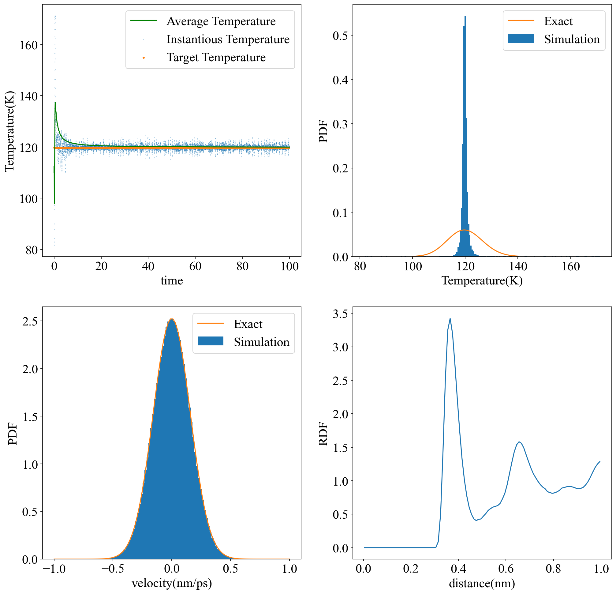
  • 20 ps 后平均温度稳定在目标温度附近,速度分布与MB分布吻合得很好
  • 经典离域子体系理想的温度分布为:

\[ f(T)=\frac{1}{\Gamma(\frac{3N+1}{2})}(\frac{3N}{2T_0})^{\frac{3N+1}{2}}\cdot T^{\frac{3N-1}{2}}\cdot exp(-\frac{3N}{2T_0}T) \]

当N很大时,上述分布区域Gauss分布,且变得尖锐。温度的相对涨落满足: \[ \frac{\sigma^2_T}{<T>^2}=\frac{2}{3N} \] 由图可见,虽然任一自由度的速度分布与理想分布十分吻合,模拟产生的温度分布相比理想情形过于尖锐。调节热浴质量参数可能使温度涨落更接近理想。

  • 径向分布函数在LJ势的极小值点附近出现第一个极大值,与实际情况吻合。由于模拟时长较短,曲线不够平滑。最大距离不能超过模拟盒子的一半长度,以免计算粒子与自身镜像的作用,因而此处无法显示 1.5 nm 附近RDF趋于1的情况。
1
2
3
4
5
6
7
8
9
10
11
12
13
14
15
16
17
18
19
20
21
22
23
24
25
26
27
28
29
30
31
32
33
34
35
36
37
38
39
40
41
42
43
44
45
46
47
48
49
50
51
52
53
54
%matplotlib inline 
from math import gamma
nstep=10000
plt.rcParams["font.family"]=['Times New Roman']
plt.rcParams["font.size"]=20
#分析1.温度随时间的变化
plt.figure(figsize=[16,16],dpi=150)
plt.subplot(221)
plt.xlabel("time")
plt.ylabel("Temperature(K)")
avT=np.zeros(nstep+1)
for n in np.arange(nstep+1):
avT[n]=sum(Ts[0:n+1])/(n+1)
plt.scatter(times,Ts,label="Instantious Temperature",marker='p',alpha=0.5,s=0.1)
plt.plot(times,avT,label="Average Temperature",color='g')
plt.scatter(times[0:nstep:20],T0*np.ones(nstep+1)[0:nstep:20],label="Target Temperature",s=5,marker='o')
plt.legend()
#分析2.温度的分布,与理想的平衡分布比较
plt.subplot(222)
plt.hist(Ts,bins=200,density=True,label='Simulation')
tx=np.linspace(100,140,100)

te=np.power(3*N/(2*pi*T0*tx),0.5)
for i in np.arange(0.5*3*N):
te*=3*N*tx/2/T0*np.exp(-tx/T0)/(0.5+i)

plt.plot(tx,te,label='Exact')
plt.xlabel("Temperature(K)")
plt.ylabel("PDF")
plt.legend()
#分析3.速度的分布,与理想的平衡分布(高斯分布)比较
with open('LJsim1_vstore.pickle', 'rb') as f:
vstore2 = pickle.load(f)
plt.subplot(223)
plt.xlabel("velocity(nm/ps)")
plt.ylabel("PDF")
plt.hist(np.ravel(vstore2),bins=100, density=True,label='Simulation')
vx=np.linspace(-1,1,100)
ve=sqrt(m[0]/(2*pi*k*T0))*np.exp(-0.5*m[0]*vx**2/k/T0)
plt.plot(vx,ve,label='Exact')
plt.legend(loc='upper right')
#分析4:径向分布函数
plt.subplot(224)

with open('LJsim1_xstore.pickle', 'rb') as f:
xstore2 = pickle.load(f)
#RDF(xtrj,rmax,nr)
[disr,rdf]=RDF(xstore2[0:10001:10],1.0,100)

plt.xlabel("distance(nm)")
plt.ylabel("RDF")
plt.plot(disr,rdf)

plt.show()

参考文献

  1. Mark E. Tuckerman. (2010). Statistical Mechanics: Theory and Molecular Simulation. Oxford: Oxford University Press.

  2. Daan Frenkel & Berend Smit著, 汪文川译. (2002). 分子模拟:从算法到应用. 化学工业出版社.


A Python Demo for MD simulation of Lennard-Jones Fluid in NVT Ensemble
http://example.com/2024/02/11/LJ-fluid-simulation/
Author
Graminilune
Posted on
February 11, 2024
Licensed under